Data Manipulation with dplyr

Overview

Teaching: 60 min
Exercises: 30 min

Questions

Objectives

Select certain columns in a data frame with the dplyr function select().

Extract certain rows in a data frame according to logical (boolean) conditions with the dplyr function filter().

Link the output of one dplyr function to the input of another function with the ‘pipe’ operator %>%.

Combine data frames using dplyr *_join() functions.

Arrange the dataset by one or multiple variables with dplyr function arrange().

Export a data frame to a .csv file.

Our biological question: do our favourite genes change expression in this dataset?

This workshop is based around a common situation in transcriptomics. We are interested in a group of genes, and another study has measured expression in conditions where expression of these genes might be interesting. Can we tell if our favourite genes have changing expression?

Here the dataset is of cell cycle progression in the yeast Saccharomyces cerevisiae, from this paper: Translational control of lipogenic enzymes in the cell cycle of synchronous, growing yeast cells. Blank et al. 2017 https://doi.org/10.15252/embj.201695050.

Fig 2 from Blank et al. 2017

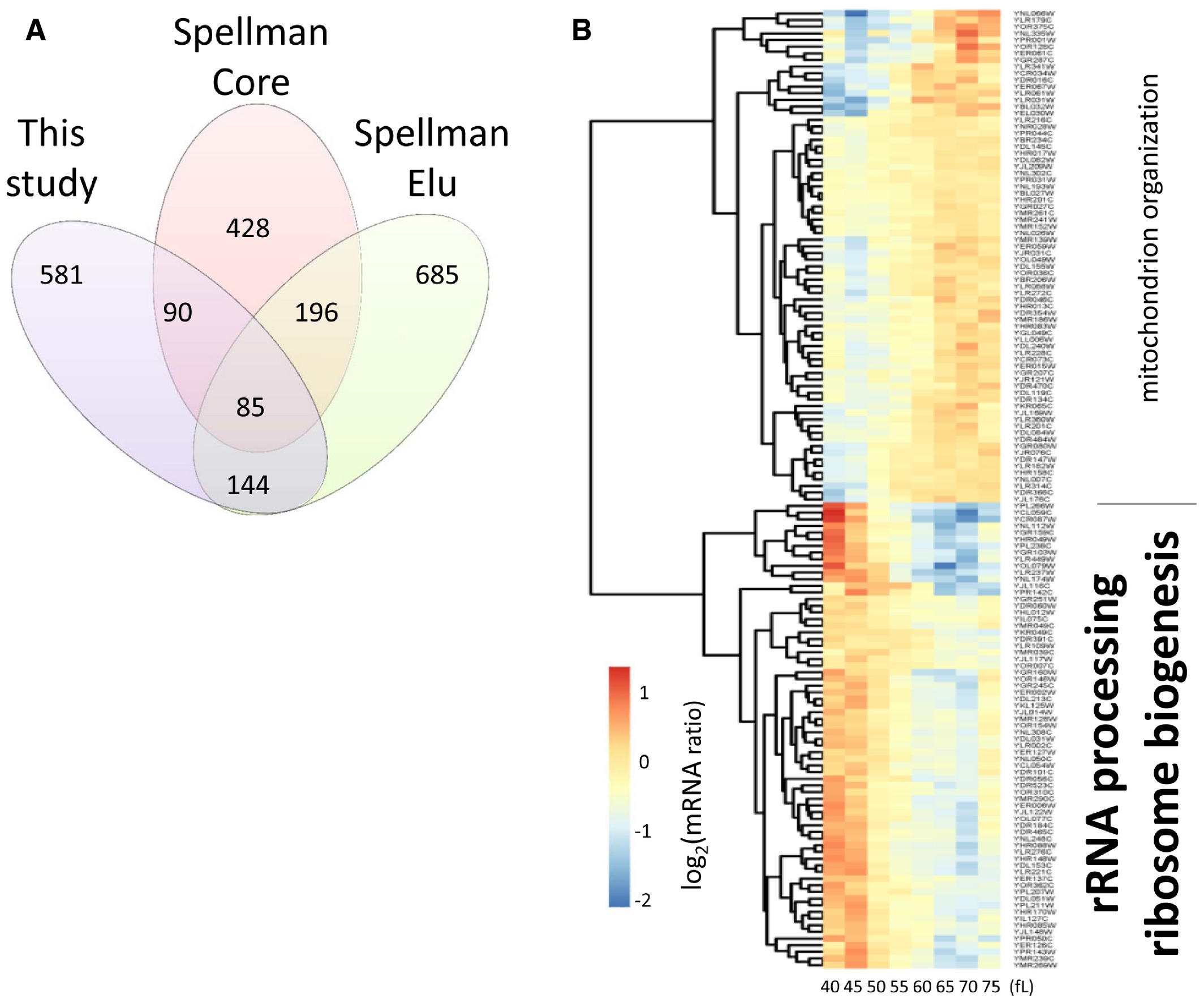
In Figure 2, the paper notes that ribosome biogenesis genes are periodically expressed during the cell cycle, but doesn’t tell us which ones.

Can we find if our favourite gene is indeed periodically expressed?

So our data analysis goals are:

Find which ribosome biogenesis genes are on the list in figure 2
Is our favourite gene NOP56 (fibrillarin, required for assembly of the 60S ribosomal sub-unit!) periodically expressed?

In another lesson, we will then carry on using this data to:

Recreate figure 2 so we can read the gene names.

These goals teach common tasks in analysing tabular data:

compare two tables, to find which elements are in both tables (here, genes)
extract/filter a small portion of a large dataset for closer inspection
use two different names for related objects (here, systematic ORF IDs and gene names)

This last point is extremely common in bioinformatics, where there are entrez gene IDs, uniprot protein IDs, etc. Often “in the wild” we need to take one set of data labeled with one ID, and compare it to another set of data labeled with a different ID. Tools in R and the tidyverse can help with that.

Data Manipulation using tidyverse

Packages in R are basically sets of additional functions that let you do more stuff. The functions we’ve been using so far, like str(), come built into R; packages give you access to more of them. Before you use a package for the first time you need to install it on your machine, and then you should import it in every subsequent R session when you need it. You should already have installed the tidyverse package. This is an “umbrella-package” that installs several packages useful for data analysis which work together well such as readr, tidyr, dplyr, ggplot2, tibble, etc.

The tidyverse package tries to address 3 common issues that arise when doing data analysis with some of the functions that come with R:

The results from a base R function sometimes depend on the type of data.
Using R expressions in a non standard way, which can be confusing for new learners.
Hidden arguments, having default operations that new learners are not aware of.

To load the package type:

## load the tidyverse packages, incl. dplyr
library("tidyverse")

What are `readr`, `dplyr` and `tidyr`?

We’ll read in our data using read_lines() and read_tsv() functions, from the tidyverse package readr.

The package dplyr provides easy tools for the most common data manipulation tasks. It is built to work directly with data frames, with many common tasks optimized by being written in a compiled language (C++). An additional feature is the ability to work directly with data stored in an external database. The benefits of doing this are that the data can be managed natively in a relational database, queries can be conducted on that database, and only the results of the query are returned.

This addresses a common problem with R in that all operations are conducted in-memory and thus the amount of data you can work with is limited by available memory. The database connections essentially remove that limitation in that you can connect to a database of many hundreds of GB, conduct queries on it directly, and pull back into R only what you need for analysis.

The package tidyr addresses the common problem of wanting to reshape your data for plotting and use by different R functions. Sometimes we want data sets where we have one row per measurement. Sometimes we want a data frame where each measurement type has its own column, and rows are instead more aggregated groups

like plots or aquaria. Moving back and forth between these formats is non-trivial, and tidyr gives you tools for this and more sophisticated data manipulation.

To learn more about dplyr and tidyr after the workshop, you may want to check out this handy data transformation with dplyr cheatsheet and this one about tidyr.

Which ribosome biogenesis genes are in the list?

We need the list from figure 2 of the paper, and a list of ribosomal biogenesis (ribi) genes.

List of genes from figure 2 in the paper

The paper says:

> * We then used the log2-transformations of these ratio values as input (see Fig 2 and Dataset 1 within the Source Data for this figure; also deposited in GEO:GSE81932).
> * Heatmap of the mRNA levels of the 144 genes (Dataset 2 within the Source Data for this figure) in common between the “Spellman Elu” and “This study” datasets.

This tells us that there are two sources for the data, one at the journal website and the other at NCBI’s Gene Expression Omnibus. We can now search GEO:GSE81932, and see the website: https://www.ncbi.nlm.nih.gov/geo/query/acc.cgi?acc=GSE81932

And at the bottom, there is GSE81932_Dataset02.txt.gz. Let’s download that, using a function called read_lines().

# get the help page for read_lines()
?read_lines

The help tells us about an n_max argument that controls how many lines we read. This is useful to inspect a file to see what it looks like before getting started. These functions can read data directly from online URLs, and automatically deal with compressed .gz files, which is very useful.

It will be easier if we make the file location an object rather than having to type it repeatedly. So let’s read the first few lines of the file to check what it contains:

# create an object to hold our file location
periodically_expressed_genes_file <- "ftp://ftp.ncbi.nlm.nih.gov/geo/series/GSE81nnn/GSE81932/suppl/GSE81932_Dataset02.txt.gz"

# show the first 10 lines of the file (using the file location object)
read_lines(periodically_expressed_genes_file, n_max = 10)

 [1] "YBL027W" "YBL032W" "YBR206W" "YBR234C" "YCL054W" "YCL059C" "YCR034W"
 [8] "YCR073C" "YCR087W" "YDL031W"

The output looks like a character vector containing gene names, which is what we want, so let’s load that into an object in our workspace by removing the n_max argument from our previous read_lines() function and assigning it to a name for our object (“periodically_expressed_genes”).

# create a data object by reading the whole file contents in
periodically_expressed_genes <- read_lines(periodically_expressed_genes_file)

Now we have the list of genes which were found to be periodically expressed in the study.

Challenge:

How many genes are on the list?

Can you see the last genes in the list?
Solution

How many genes are on the list?
length(periodically_expressed_genes)
[1] 144
Can you see the last genes in the list?
tail(periodically_expressed_genes)
[1] "YPR001W" "YPR031W" "YPR044C" "YPR050C" "YPR142C" "YPR143W"

List of ribosomal biogenesis (ribi) genes.

For this lesson, we will use the list of yeast ribi genes from the Saccharomyces Genome Database (SGD) Gene Ontology information, which can be found at: yeastgenome.org/go/GO:0042254

Go to the bottom of the page for the longer computational list, click download and place the file in your data directory. You’ll need to have a folder on your machine called “data” where you’ll download the file.

Now we can take a look at it in R.

We are going to use the tidyverse function read_tsv() to read the contents of this file into R as a tibble (nice data frame) object. Inside the read_tsv() command, the first entry is a character string with the file name (“data/ribosome_biogenesis_annotations.txt”)

ribi_annotation_file <- "data/ribosome_biogenesis_annotations.txt"

read_lines(ribi_annotation_file, n_max = 10)

 [1] "!"                                                                                                                                                               
 [2] "!Date: 04/23/2019"                                                                                                                                               
 [3] "!From: Saccharomyces Genome Database (SGD) "                                                                                                                     
 [4] "!URL: http://www.yeastgenome.org/ "                                                                                                                              
 [5] "!Contact Email: sgd-helpdesk@lists.stanford.edu "                                                                                                                
 [6] "!Funding: NHGRI at US NIH, grant number 5-U41-HG001315 "                                                                                                         
 [7] "!"                                                                                                                                                               
 [8] ""                                                                                                                                                                
 [9] "Gene\tGene Systematic Name\tQualifier\tGene Ontology Term ID\tGene Ontology Term\tAspect\tAnnotation Extension\tEvidence\tMethod\tSource\tAssigned On\tReference"
[10] "ECM1\tYAL059W\tribosome biogenesis\tGO:0042254\t\tbiological process\tIEA with KW-0690\tcomputational\tUniProt\t2019-04-20\t\tUniProt-GOA (2011)"                

What does this tell us about the file? It is a text file, the first few lines start with a ! character, and afterwards the tab-delimited table starts with tabs encoded as \t.

We can remove the unwanted lines in two ways. We can either skip them:

read_tsv(ribi_annotation_file, skip = 7)

Parsed with column specification:
cols(
  Gene = col_character(),
  `Gene Systematic Name` = col_character(),
  Qualifier = col_character(),
  `Gene Ontology Term ID` = col_character(),
  `Gene Ontology Term` = col_logical(),
  Aspect = col_character(),
  `Annotation Extension` = col_character(),
  Evidence = col_character(),
  Method = col_character(),
  Source = col_date(format = ""),
  `Assigned On` = col_logical(),
  Reference = col_character()
)

# A tibble: 218 x 12
   Gene  `Gene Systemati… Qualifier `Gene Ontology … `Gene Ontology … Aspect
   <chr> <chr>            <chr>     <chr>            <lgl>            <chr> 
 1 ECM1  YAL059W          ribosome… GO:0042254       NA               biolo…
 2 UTP20 YBL004W          ribosome… GO:0042254       NA               biolo…
 3 MAK5  YBR142W          ribosome… GO:0042254       NA               biolo…
 4 RPB5  YBR154C          ribosome… GO:0042254       NA               biolo…
 5 RPS6B YBR181C          ribosome… GO:0042254       NA               biolo…
 6 RPS9B YBR189W          ribosome… GO:0042254       NA               biolo…
 7 ENP1  YBR247C          ribosome… GO:0042254       NA               biolo…
 8 REI1  YBR267W          ribosome… GO:0042254       NA               biolo…
 9 RRP7  YCL031C          ribosome… GO:0042254       NA               biolo…
10 SPB1  YCL054W          ribosome… GO:0042254       NA               biolo…
# … with 208 more rows, and 6 more variables: `Annotation Extension` <chr>,
#   Evidence <chr>, Method <chr>, Source <date>, `Assigned On` <lgl>,
#   Reference <chr>

Or we can tell R that the ! is a comment character, and lines after that should be ignored.

read_tsv(ribi_annotation_file, comment = "!")

Parsed with column specification:
cols(
  Gene = col_character(),
  `Gene Systematic Name` = col_character(),
  Qualifier = col_character(),
  `Gene Ontology Term ID` = col_character(),
  `Gene Ontology Term` = col_logical(),
  Aspect = col_character(),
  `Annotation Extension` = col_character(),
  Evidence = col_character(),
  Method = col_character(),
  Source = col_date(format = ""),
  `Assigned On` = col_logical(),
  Reference = col_character()
)

# A tibble: 218 x 12
   Gene  `Gene Systemati… Qualifier `Gene Ontology … `Gene Ontology … Aspect
   <chr> <chr>            <chr>     <chr>            <lgl>            <chr> 
 1 ECM1  YAL059W          ribosome… GO:0042254       NA               biolo…
 2 UTP20 YBL004W          ribosome… GO:0042254       NA               biolo…
 3 MAK5  YBR142W          ribosome… GO:0042254       NA               biolo…
 4 RPB5  YBR154C          ribosome… GO:0042254       NA               biolo…
 5 RPS6B YBR181C          ribosome… GO:0042254       NA               biolo…
 6 RPS9B YBR189W          ribosome… GO:0042254       NA               biolo…
 7 ENP1  YBR247C          ribosome… GO:0042254       NA               biolo…
 8 REI1  YBR267W          ribosome… GO:0042254       NA               biolo…
 9 RRP7  YCL031C          ribosome… GO:0042254       NA               biolo…
10 SPB1  YCL054W          ribosome… GO:0042254       NA               biolo…
# … with 208 more rows, and 6 more variables: `Annotation Extension` <chr>,
#   Evidence <chr>, Method <chr>, Source <date>, `Assigned On` <lgl>,
#   Reference <chr>

Because we will need to reuse this data, let’s make it into an object.

ribi_annotation <- read_tsv(ribi_annotation_file, comment = "!")

Parsed with column specification:
cols(
  Gene = col_character(),
  `Gene Systematic Name` = col_character(),
  Qualifier = col_character(),
  `Gene Ontology Term ID` = col_character(),
  `Gene Ontology Term` = col_logical(),
  Aspect = col_character(),
  `Annotation Extension` = col_character(),
  Evidence = col_character(),
  Method = col_character(),
  Source = col_date(format = ""),
  `Assigned On` = col_logical(),
  Reference = col_character()
)

This statement doesn’t show any of the data as output because, as you might recall, assignments don’t display anything. If we want to check that our data has been loaded, we can see the contents of the data frame by typing its name: ribi_annotation, or using the view() command.

# view the data object
ribi_annotation

## try also:
View(ribi_annotation)

At this point it’s also worth checking the structure of our dataset using str() to find out whether it’s what we’d expect, and look at what modes of data it contains.

# check structure of the data
str(ribi_annotation)

tibble [218 × 12] (S3: spec_tbl_df/tbl_df/tbl/data.frame)
 $ Gene                 : chr [1:218] "ECM1" "UTP20" "MAK5" "RPB5" ...
 $ Gene Systematic Name : chr [1:218] "YAL059W" "YBL004W" "YBR142W" "YBR154C" ...
 $ Qualifier            : chr [1:218] "ribosome biogenesis" "ribosome biogenesis" "ribosome biogenesis" "ribosome biogenesis" ...
 $ Gene Ontology Term ID: chr [1:218] "GO:0042254" "GO:0042254" "GO:0042254" "GO:0042254" ...
 $ Gene Ontology Term   : logi [1:218] NA NA NA NA NA NA ...
 $ Aspect               : chr [1:218] "biological process" "biological process" "biological process" "biological process" ...
 $ Annotation Extension : chr [1:218] "IEA with KW-0690" "IEA with KW-0690" "IEA with KW-0690" "IEA with KW-0690" ...
 $ Evidence             : chr [1:218] "computational" "computational" "computational" "computational" ...
 $ Method               : chr [1:218] "UniProt" "UniProt" "UniProt" "UniProt" ...
 $ Source               : Date[1:218], format: "2019-04-20" "2019-04-20" ...
 $ Assigned On          : logi [1:218] NA NA NA NA NA NA ...
 $ Reference            : chr [1:218] "UniProt-GOA (2011)" "UniProt-GOA (2011)" "UniProt-GOA (2011)" "UniProt-GOA (2011)" ...
 - attr(*, "spec")=
  .. cols(
  ..   Gene = col_character(),
  ..   `Gene Systematic Name` = col_character(),
  ..   Qualifier = col_character(),
  ..   `Gene Ontology Term ID` = col_character(),
  ..   `Gene Ontology Term` = col_logical(),
  ..   Aspect = col_character(),
  ..   `Annotation Extension` = col_character(),
  ..   Evidence = col_character(),
  ..   Method = col_character(),
  ..   Source = col_date(format = ""),
  ..   `Assigned On` = col_logical(),
  ..   Reference = col_character()
  .. )

Now we have our data in R, we’re going to learn how to inspect it more thoroughly, and manipulate it using some of the most common dplyr functions:

select(): subset columns
n_distinct() and distinct(): count or filter unique rows
filter(): subset rows on conditions
mutate(): create new columns by using information from other columns
group_by() and summarize(): create summary statistics on grouped data
arrange(): sort results
count(): count discrete values

What’s in a name?

Our ribi_annotation object contains a lot of extra information we won’t be using, but it all relates to what different genes are annotated as, and how they relate to other genes.

Two of the variables in our object (Gene and Gene Systematic Name) are particularly useful when it comes to answering our questions about which genes were shown in Figure 2, and whether our ‘favourite gene’ NOP56 was periodically expressed.

Gene holds the shorter more familiar Gene Names, while Gene Systematic Name contains the more ‘official’ name but is less helpful in telling us what that gene actually does.

We can also see from the results of str() that the Qualifier field holds information on what kind of genes these are.

Because we’ve downloaded this set of Gene Ontology records from the page for “Ribosome Biogenesis”, we might expect that to be the only type of genes we’ve got in this data object, so let’s check using the dplyr::n_distinct() function and the dplyr::distinct() function:

# how many (e.g. n) distinct entries for Qualifier?
n_distinct(ribi_annotation$Qualifier)

[1] 1

# show distinct (unique) entries
distinct(ribi_annotation, Qualifier)

# A tibble: 1 x 1
  Qualifier          
  <chr>              
1 ribosome biogenesis

We can see that the answer to n_distinct(ribi_annotation$Qualifier) is 1, which is what we thought. We use can distinct(ribi_annotation, Qualifier) to confirm that, and show us what that unique entry is (“ribosome biogenesis”).

NOTE: You may have noticed that the format of these two commands is slightly different. For distinct(), we’ve provided TWO arguments (the data object and the variable name from that object), while for n_distinct() we’ve only provided one (the data object with the variable accessed via the $ symbol, a common way of accessing variables in data frames). You can look at the help information for both functions (e.g. ?n_distinct) to see why this is.
n_distinct() requires a vector of values as its main argument, whereas distinct() takes a data object (e.g. our tibble / data frames) and can then take optional variables to use when determining uniqueness - so here we’ve checked for unique rows from the Qualifier column.

Now we want to pull out (select!) just the columns from ribi_annotation that we’re interested in taking data from (Gene and Gene Systematic Name).

We can do this with the dplyr::select() function:

# pull out short informal gene names column and longer systematic names column as separate objet
ribi_annotation_names <- select(ribi_annotation, Gene, SystematicName = "Gene Systematic Name")

# check structure
str(ribi_annotation_names)

tibble [218 × 2] (S3: tbl_df/tbl/data.frame)
 $ Gene          : chr [1:218] "ECM1" "UTP20" "MAK5" "RPB5" ...
 $ SystematicName: chr [1:218] "YAL059W" "YBL004W" "YBR142W" "YBR154C" ...

Here we can see that we now have an object of 2 columns, containing the same number of rows as our original. Great.

But is 218 the real number of unique genes? Or are there duplicates? Let’s use n_distinct() and distinct() to make sure we’ve got no replicated names.

# check number of distinct gene name & systematic name combos
n_distinct(ribi_annotation_names)

[1] 187

Using n_distinct(), we can see that this is a smaller number than before, so there ARE some duplicates we can weed out. This is where distinct() comes in:

# create new object without duplicated rows of Gene Names & Systematic Names
ribi_genes <- distinct(ribi_annotation_names)

Perfect!

So which ribi genes are periodically expressed?

Now we know which genes are ribi genes, and we know which genes were periodically expressed, how can we check which ribi genes are periodically expressed?

We can use filter(), combined with a handy operator %in%.

TIP: if you want to find the help page for special symbolic operators like %in%, you’ll need to wrap them in quotes when searching: e.g. ?"%in%" or you’ll end up with an error saying “unexpected SPECIAL”.

Applying the filter() function on our ribi_genes object, we can return the rows where the systematic name appears in the periodically_expressed_genes object:

filter(ribi_genes, SystematicName %in% periodically_expressed_genes)

# A tibble: 34 x 2
   Gene  SystematicName
   <chr> <chr>         
SPB1  YCL054W       
KRR1  YCL059C       
DBP10 YDL031W       
SAS10 YDL153C       
NOP6  YDL213C       
MAK21 YDR060W       
NOP16 YER002W       
NUG1  YER006W       
NSA2  YER126C       
LCP5  YER127W       
# … with 24 more rows

So, it seems that plenty of these ribi (ribosome biogenesis) genes are periodically expressed during the cell cycle! Mission accomplished.

Find all gene names and IDs

In the above section, we used the ribi_annotation_names data to compare gene names (e.g. NOP56) with systematic IDs given in another dataset (e.g. YLR197W), but only for ribosomal biogenesis genes. Here, it will be helpful to do find gene names for all genes regardless of function.

Usually the first step is to find a file in an archive with both sets of names. Today, we will use a file with yeast gene names, systematic IDs, and abundance information in a tidy format, from the Dryad Data Repository here.

Download the dataset from the “Data Files” section on the right-hand side of the page. This will download a zip file to your local computer. Extract the files within to somewhere sensible.

Copy or move the file scer-mrna-protein-absolute-estimate.txt to the data/ folder in the working directory R is using. If you don’t have a data/ folder in your working directory, create it. If you’re working in Notable RStudio Server, you’ll have to download the files locally, extract them, then upload the relevant file to your R working directory on the server.

Again, we don’t know immediately what the format of this text-based file will be, so we can use read_lines() to suss things out:

scer_names_estimates_file <- "../data/scer-mrna-protein-absolute-estimate.txt"

# read first 10 lines
read_lines(scer_names_estimates_file, n_max = 10)

 [1] "# SCM estimates of absolute mRNA and protein levels, scaled to (average) molecules per haploid cell, for haploid budding yeast (S.cerevisiae) growing exponentially in rich medium with glucose "
 [2] "#"                                                                                                                                                                                               
 [3] "# Generated Tue Apr 07 00:00:36 2015 "                                                                                                                                                           
 [4] "#"                                                                                                                                                                                               
 [5] "# Citation:"                                                                                                                                                                                     
 [6] "#   \"Accounting for experimental noise reveals that transcript levels,"                                                                                                                         
 [7] "#   amplified by post-transcriptional regulation, largely determine steady-state protein levels in yeast,\""                                                                                     
 [8] "#   Gábor Csárdi, Alexander Franks, David S. Choi, Eduardo M. Airoldi, and D. Allan Drummond, PLoS Genetics, 2015"                                                                               
 [9] "#"                                                                                                                                                                                               
[10] "# orf = Systematic yeast ORF (open reading frame) identifier"                                                                                                                                    

Here we can see that this file uses the # symbol to represent comments, so we can read in the file, adding a comment = "#" argument to our function:

# read in file and save as object:
scer_names_estimates <- read_tsv(scer_names_estimates_file, comment = "#")

Parsed with column specification:
cols(
  orf = col_character(),
  gene = col_character(),
  mrna = col_double(),
  prot = col_double(),
  sd.mrna = col_double(),
  sd.prot = col_double(),
  n.mrna = col_double(),
  n.prot = col_double()
)

Now we’ve read the data in, it’s good to take a quick check of the structure using str().

str(scer_names_estimates)

tibble [5,887 × 8] (S3: spec_tbl_df/tbl_df/tbl/data.frame)
 $ orf    : chr [1:5887] "Q0045" "Q0050" "Q0055" "Q0060" ...
 $ gene   : chr [1:5887] "COX1" "AI1" "AI2" "AI3" ...
 $ mrna   : num [1:5887] 0.1835 0.0967 0.0655 0.0669 0.0666 ...
 $ prot   : num [1:5887] 18.44 4.67 3.94 2.38 2.18 ...
 $ sd.mrna: num [1:5887] 0.333 0.414 0.462 0.443 0.394 0.472 0.404 0.393 0.325 0.36 ...
 $ sd.prot: num [1:5887] 0.371 0.48 0.533 0.541 0.528 0.61 0.474 0.464 0.451 0.467 ...
 $ n.mrna : num [1:5887] 3 2 2 2 2 2 2 2 3 3 ...
 $ n.prot : num [1:5887] 2 1 1 1 0 0 0 0 1 1 ...
 - attr(*, "spec")=
  .. cols(
  ..   orf = col_character(),
  ..   gene = col_character(),
  ..   mrna = col_double(),
  ..   prot = col_double(),
  ..   sd.mrna = col_double(),
  ..   sd.prot = col_double(),
  ..   n.mrna = col_double(),
  ..   n.prot = col_double()
  .. )

We can tell from the output of str(scer_names_estimates) that the columns we’re interested in which can help us answer our questions are likely to be orf and gene since these are the gene names we’re after.

Let’s pull out these relevant columns again, using select(), but let’s make the new column names in our new table the same as those we’ve extracted from the ribi_annotation_names table:

# create a new data object and rename the columns for the new table:
scer_gene_names <- select(scer_names_estimates, Gene = gene, SystematicName = orf)

A quick check of str() or dim() on this new object and you can see we’ve got the right dimensions on our new table.

Challenge:

How would we find the names of the genes on the list of periodically expressed genes?
How would we then extract only the shorter gene names from the output in Challenge 1.?
Is NOP56 on the list?

Solution

filter(scer_gene_names, SystematicName %in% periodically_expressed_genes)

# A tibble: 132 x 2
   Gene   SystematicName
   <chr>  <chr>         
RPL19B YBL027W       
HEK2   YBL032W       
ARC40  YBR234C       
SPB1   YCL054W       
KRR1   YCL059C       
ELO2   YCR034W       
SSK22  YCR073C       
DBP10  YDL031W       
LHP1   YDL051W       
RPL13A YDL082W       
# … with 122 more rows

filter(scer_gene_names, SystematicName %in% periodically_expressed_genes) %>% select(Gene)

# A tibble: 132 x 1
   Gene  
   <chr> 
RPL19B
HEK2  
ARC40 
SPB1  
KRR1  
ELO2  
SSK22 
DBP10 
LHP1  
RPL13A
# … with 122 more rows

filter(scer_gene_names, SystematicName %in% periodically_expressed_genes, Gene == "NOP56")

# A tibble: 0 x 2
# … with 2 variables: Gene <chr>, SystematicName <chr>

No, NOP56 is not on the list. We can double-check that NOP56 is on the list of scer_gene_names by:

filter(scer_gene_names, Gene == "NOP56")

# A tibble: 1 x 2
  Gene  SystematicName
  <chr> <chr>         
1 NOP56 YLR197W       

which it is. But, NOP56’s gene ID “YLR197W” is not on the list of periodically_expressed_genes. We can double-check this by

"YLR197W" %in% periodically_expressed_genes

[1] FALSE

Sorting our datasets with `arrange()`

Often, we want to view data to emphasize one variable or another. For example, we might want to find the genes with highest abundance in one dataset. To achieve this, we order the rows of our data frame, using the dplyr::arrange() function in ascending and descending order on one or more variables.

Let’s try that on our scer_names_estimates table:

# arrange by `gene` 
arrange(scer_names_estimates, gene)

# A tibble: 5,887 x 8
   orf     gene    mrna    prot sd.mrna sd.prot n.mrna n.prot
   <chr>   <chr>  <dbl>   <dbl>   <dbl>   <dbl>  <dbl>  <dbl>
YMR056C AAC1   1.17    176.    0.286   0.402     11      1
YBR085W AAC3   2.50    851.    0.235   0.283     11      3
YJR155W AAD10  0.744    69.6   0.289   0.418     10      0
YNL331C AAD14  0.910    83.3   0.325   0.464      8      0
YOL165C AAD15  0.669    57.8   0.324   0.473     10      0
YCR107W AAD3   0.893    84.8   0.289   0.395      7      1
YDL243C AAD4   1.08    103.    0.292   0.42       8      0
YFL056C AAD6   0.673    62.3   0.308   0.385      8      0
YNL141W AAH1  10.4   10787.    0.27    0.199     13      6
YHR047C AAP1   5.08   3188.    0.246   0.215      9      8
# … with 5,877 more rows

# show tail() of dataset
arrange(scer_names_estimates, gene) %>% tail()

# A tibble: 6 x 8
  orf     gene   mrna   prot sd.mrna sd.prot n.mrna n.prot
  <chr>   <chr> <dbl>  <dbl>   <dbl>   <dbl>  <dbl>  <dbl>
1 YPR172W <NA>  3.23  1068.    0.255   0.222     12      8
2 YPR174C <NA>  2.26   957.    0.268   0.223     11      4
3 YPR196W <NA>  0.697   69.0   0.32    0.39       9      0
4 YPR202W <NA>  0.475   37.8   0.305   0.408      5      0
5 YPR203W <NA>  0.268   16.9   0.35    0.457      5      0
6 YPR204W <NA>  1.04   116.    0.304   0.436      5      0

# arrange by `gene` in DESCENDING order and `mrna` in ASCENDING order.
arrange(scer_names_estimates, desc(gene), mrna)

# A tibble: 5,887 x 8
   orf     gene    mrna   prot sd.mrna sd.prot n.mrna n.prot
   <chr>   <chr>  <dbl>  <dbl>   <dbl>   <dbl>  <dbl>  <dbl>
YNL241C ZWF1   8.71  12312.   0.266   0.212     12     10
YGR285C ZUO1  36.1   65470.   0.227   0.239     12      9
YBR046C ZTA1   4.53   1790.   0.262   0.269     11      7
YKL175W ZRT3   5.76   1023.   0.26    0.32      11      2
YLR130C ZRT2   4.62   1522.   0.242   0.276     12      3
YGL255W ZRT1   3.62    696.   0.261   0.387     12      1
YER033C ZRG8   0.994   164.   0.281   0.34       9      3
YNR039C ZRG17  3.24    892.   0.267   0.253     12      3
YMR243C ZRC1  14.9    9208.   0.216   0.237     13      4
YOL154W ZPS1   0.953   124.   0.283   0.439     10      1
# … with 5,877 more rows

# show tail() of dataset (arranged by `gene` in DESCENDING order and `mrna` in ASCENDING order)
arrange(scer_names_estimates, desc(gene), mrna) %>% tail()

# A tibble: 6 x 8
  orf       gene   mrna  prot sd.mrna sd.prot n.mrna n.prot
  <chr>     <chr> <dbl> <dbl>   <dbl>   <dbl>  <dbl>  <dbl>
1 YOR192C-A <NA>     NA    NA      NA      NA      0      0
2 YOR343W-A <NA>     NA    NA      NA      NA      0      0
3 YPL257W-A <NA>     NA    NA      NA      NA      0      0
4 YPR137C-A <NA>     NA    NA      NA      NA      0      0
5 YPR158C-C <NA>     NA    NA      NA      NA      0      0
6 YPR158W-A <NA>     NA    NA      NA      NA      0      0

One of the key things that arrange() does differently from the base R sort() function, is that NA values (ie missing values) are always sorted to the END of the data, regardless of whether you’ve sorted by ascending (the default) or descending order (using the desc() function around the relevant variable).

What is NOP56 doing?

The paper reported that NOP56 is not periodically expressed during the cell cycle. We can go on to look in more depth at that gene specifically, to find what it is doing.

We can now read in Dataset 1 from the Blank et al. paper:

We then used the log2-transformations of these ratio values as input (see Fig 2 and Dataset 1 within the Source Data for this figure; also deposited in GEO:GSE81932).

… which we found the link for via the accession number GEO:GSE81932, at NCBI’s Gene Expression Omnibus website: https://www.ncbi.nlm.nih.gov/geo/query/acc.cgi?acc=GSE81932.

This file contains mRNA levels for each gene at specific measured cell sizes (in femtoLitres), and so represents gene expression divided by cell size. Since we know cells will grow larger through the cell cycle, we can orient ourselves about what’s happening for a particular gene such as NOP56.

We can use read_tsv() in the same way as earlier:

# download the mRNA data 
mRNA_data <- read_tsv("ftp://ftp.ncbi.nlm.nih.gov/geo/series/GSE81nnn/GSE81932/suppl/GSE81932_Dataset01.txt.gz")

Parsed with column specification:
cols(
  ORF = col_character(),
  `40 fL` = col_double(),
  `45 fL` = col_double(),
  `50 fL` = col_double(),
  `55 fL` = col_double(),
  `60 fL` = col_double(),
  `65 fL` = col_double(),
  `70 fL` = col_double(),
  `75 fL` = col_double()
)

# check structure
str(mRNA_data)

tibble [6,713 × 9] (S3: spec_tbl_df/tbl_df/tbl/data.frame)
 $ ORF  : chr [1:6713] "Q0010" "Q0017" "Q0032" "Q0045" ...
 $ 40 fL: num [1:6713] 0.145 -1.324 NA 0.252 -0.784 ...
 $ 45 fL: num [1:6713] -0.421 -0.711 NA -0.339 -0.635 ...
 $ 50 fL: num [1:6713] NA 0.317 NA -0.595 -0.622 ...
 $ 55 fL: num [1:6713] -1.257 0.618 NA -0.281 -0.222 ...
 $ 60 fL: num [1:6713] -1.4798 -0.4981 NA -0.6327 -0.0648 ...
 $ 65 fL: num [1:6713] -0.111 0.208 2.566 0.469 0.76 ...
 $ 70 fL: num [1:6713] 1.154 0.075 1.057 0.631 0.766 ...
 $ 75 fL: num [1:6713] 1.1496 0.3716 NA -0.0643 -0.1239 ...
 - attr(*, "spec")=
  .. cols(
  ..   ORF = col_character(),
  ..   `40 fL` = col_double(),
  ..   `45 fL` = col_double(),
  ..   `50 fL` = col_double(),
  ..   `55 fL` = col_double(),
  ..   `60 fL` = col_double(),
  ..   `65 fL` = col_double(),
  ..   `70 fL` = col_double(),
  ..   `75 fL` = col_double()
  .. )

When you check the struture, you can see the measurement variables (ie. 40, 45, 50 femtoLitres etc) and you can see the variable ORF.

We can rename ORF to SystematicName to help us mentally (and programmatically!) compare and link our different datasets.

# rename ORF column
names(mRNA_data)[1] <- "SystematicName"

Joining datasets

Since we now have a column in common between our mRNA_data data frame and our scer_gene_names data frame, we can know show some the results when we look at the mRNA_data table.

All we need to do now is add the gene names column which shows us which Systematic Name refers to NOP56, and will let us label our plots with this slightly friendlier name when we come to that later.

There are multiple *_join() functions in dplyr which can help us add columns from different datasets, filtering and matching rows based on particular keys.

You can find more information about the types of join functions in the dplyr package here.

For our purposes, we want to use one of the mutating join functions called left_join(). left_join() includes all rows in x, adding columns from y, based on a variable which is common between both datasets (this is the by = argument).

In our case, we want to keep pretty much all of the mRNA_data table, but join the shorter gene names onto it from scer_gene_names for each row where the systematic names are the same (since systematic names are a column in both tables).

# join short gene names onto mRNA data from dataset 01 on `SystematicName`
mRNA_data_named <- left_join(mRNA_data, scer_gene_names, by = "SystematicName")

# show few values from first variable
print(mRNA_data_named)

# A tibble: 6,713 x 10
   SystematicName `40 fL` `45 fL` `50 fL` `55 fL` `60 fL` `65 fL` `70 fL`
   <chr>            <dbl>   <dbl>   <dbl>   <dbl>   <dbl>   <dbl>   <dbl>
Q0010            0.145  -0.421  NA      -1.26  -1.48   -0.111   1.15  
Q0017           -1.32   -0.711   0.317   0.618 -0.498   0.208   0.0750
Q0032           NA      NA      NA      NA     NA       2.57    1.06  
Q0045            0.252  -0.339  -0.595  -0.281 -0.633   0.469   0.631 
Q0050           -0.784  -0.635  -0.622  -0.222 -0.0648  0.760   0.766 
Q0055           -0.369  -0.595  -0.670  -0.108 -0.244   0.599   0.725 
Q0060           -0.143  -0.878  -0.712  -0.341 -0.0729  0.691   0.690 
Q0065           -0.377  -1.02   -1.30   -0.139 -0.325   0.749   0.837 
Q0070           -0.439  -0.305  -0.613  -0.492  0.0846 -0.0548  0.864 
Q0075           -0.450  -0.582  -0.516  -0.199  0.0631  0.570   0.710 
# … with 6,703 more rows, and 2 more variables: `75 fL` <dbl>, Gene <chr>

# show few values from all variables
glimpse(mRNA_data_named)

Rows: 6,713
Columns: 10
$ SystematicName <chr> "Q0010", "Q0017", "Q0032", "Q0045", "Q0050", "Q0055", …
$ `40 fL`        <dbl> 0.14471060, -1.32389846, NA, 0.25175335, -0.78382236, …
$ `45 fL`        <dbl> -0.420886575, -0.711179155, NA, -0.339004468, -0.63530…
$ `50 fL`        <dbl> NA, 0.31653108, NA, -0.59549053, -0.62240119, -0.66965…
$ `55 fL`        <dbl> -1.257387843, 0.617641813, NA, -0.281424022, -0.221632…
$ `60 fL`        <dbl> -1.47978026, -0.49806141, NA, -0.63274874, -0.06478821…
$ `65 fL`        <dbl> -0.11054645, 0.20776048, 2.56559718, 0.46910266, 0.760…
$ `70 fL`        <dbl> 1.15442576, 0.07495877, 1.05658353, 0.63090631, 0.7658…
$ `75 fL`        <dbl> 1.149576356, 0.371553299, NA, -0.064268654, -0.1238608…
$ Gene           <chr> NA, NA, NA, "COX1", "AI1", "AI2", "AI3", "AI4", "AI5_A…

Now we can see that the Gene information from scer_gene_names has been joined onto the mRNA_data for each row where the SystematicName value matches, and NA has been added where there’s no equivalent value in Gene.

What about NOP56?

Now we’re in a good position to find out how NOP56 gene expression changes across the cell cycle, because we’ve got the data nicely organised and we know how to filter out what we want!

Let’s do just that and pull out the observations for NOP56:

# filter out NOP56 observations:
filter(mRNA_data_named, Gene == "NOP56")

# A tibble: 1 x 10
  SystematicName `40 fL` `45 fL` `50 fL` `55 fL` `60 fL` `65 fL` `70 fL` `75 fL`
  <chr>            <dbl>   <dbl>   <dbl>   <dbl>   <dbl>   <dbl>   <dbl>   <dbl>
1 YLR197W          0.594   0.772  0.0101  -0.209  0.0770  -0.786  -0.351   -1.02
# … with 1 more variable: Gene <chr>

We can see that the mRNA content fluctuates as the cell size increases. Interesting!

How does this compare with a couple other genes of interest, for example:

ACT1: this is the gene which codes for important structural protein Actin
NOP16: this is a gene involved in 60S ribosomal subunit biogenesis

Let’s pull all three genes out:

# filter out 3 genes of interest:
filter(mRNA_data_named, Gene %in% c("ACT1", "NOP16", "NOP56"))

# A tibble: 3 x 10
  SystematicName `40 fL` `45 fL` `50 fL` `55 fL` `60 fL` `65 fL` `70 fL` `75 fL`
  <chr>            <dbl>   <dbl>   <dbl>   <dbl>   <dbl>   <dbl>   <dbl>   <dbl>
1 YER002W          0.687   0.706  0.203  -0.0884 -0.698   -0.708  -1.05  -0.0681
2 YFL039C         -0.366  -0.940 -0.191  -0.0418 -0.0523   0.180   0.379  0.544 
3 YLR197W          0.594   0.772  0.0101 -0.209   0.0770  -0.786  -0.351 -1.02  
# … with 1 more variable: Gene <chr>

We can start to see how helpful the dplyr functions will be in subsetting our data to help our analyses and visualisation!

In a later lesson, we will discuss how to turn tables like these into plots.

Answering our questions:

Our data analysis goals were:

Find which ribosome biogenesis genes are on the list in figure 2

Is our favourite gene NOP56 (fibrillarin, required for assembly of the 60S ribosomal sub-unit!) periodically expressed?

We’ve been able to compare which genes are listed in the dataset we downloaded for figure 2 against the genes listed as playing a part in ribosome biogenesis in the Gene Ontology list on the Saccharomyces Genome Database (SGD).

We’ve found out that NOP56 is not reported to be periodically expressed, and seen how its gene expression changes across the measurement timepoints.

Saving out our data using `write_csv()`

Now we have our table of mRNA with the gene names added, we might want to keep a copy of that to potentially use in later analysis.

We can save it out to a .csv file using readr::write_csv(), with our data frame as the first argument, and the file path as the second argument:

# write file to .csv:
write_csv(mRNA_data_named, "../data/mRNA_data_with_gene_names.csv")

Key Points

Use the dplyr package to manipulate dataframes.

Use select() to choose variables from a dataframe.

Use filter() to choose data based on values.

Use joins to combine data frames.

Use arrange() to sort data frames.

Export data to .csv file.

previous episode

Exploring tabular data with R using a transcriptomic example dataset.

next episode

Data Manipulation with dplyr

Overview

Our biological question: do our favourite genes change expression in this dataset?

Data Manipulation using tidyverse

What are `readr`, `dplyr` and `tidyr`?

Which ribosome biogenesis genes are in the list?

List of genes from figure 2 in the paper

Challenge:

Solution

List of ribosomal biogenesis (ribi) genes.

What’s in a name?

So which ribi genes are periodically expressed?

Find all gene names and IDs

Challenge:

Solution

Sorting our datasets with `arrange()`

What is NOP56 doing?

Joining datasets

What about NOP56?

Answering our questions:

Saving out our data using `write_csv()`

Key Points

previous episode

next episode

previous episode

Exploring tabular data with R using a transcriptomic example dataset.

next episode

Data Manipulation with dplyr

Overview

Our biological question: do our favourite genes change expression in this dataset?

Data Manipulation using tidyverse

What are readr, dplyr and tidyr?

Which ribosome biogenesis genes are in the list?

List of genes from figure 2 in the paper

Challenge:

Solution

List of ribosomal biogenesis (ribi) genes.

What’s in a name?

So which ribi genes are periodically expressed?

Find all gene names and IDs

Challenge:

Solution

Sorting our datasets with arrange()

What is NOP56 doing?

Joining datasets

What about NOP56?

Answering our questions:

Saving out our data using write_csv()

Key Points

previous episode

next episode

What are `readr`, `dplyr` and `tidyr`?

Sorting our datasets with `arrange()`

Saving out our data using `write_csv()`